Build a Keywords Ranking Tracker with Google Sheets [Including a Free Template]
A Keywords Ranking Tracker is a tool that allows you to monitor the performance of your website (or a competitor’s site) by tracking its position in Google search results on some specific queries or keywords. By regularly checking keyword rankings, you can identify trends, overall improvements or setbacks in your SEO efforts.
Thus, monitoring keyword rankings is a fundamental step in optimizing your website for better visibility and increased organic traffic.
There are many tools on the market to monitor keywords rankings. In this article, we will teach you how to create a free Google Keywords Ranking Tracker simply from Google Sheets.
We’ll build a SEO dashboard connected and synced with Google results that outputs the ranking of your ebsite on a list of keywords.
What Is Keyword Ranking?
Keyword ranking refers to a webpage’s position in Search Engine results for a particular search query. When a user initiates a search on Google or any other search engines, the position of your webpage or any competitor’s webpages in the results defines the keyword ranking.

Given that a majority of users tend to click on the first search results they encounter, securing the top positions for a specific keyword typically results in more traffic compared to lower-ranked alternatives.
Thus, it becomes essential to monitor and track where your website stands vs the relevant keywords for your audience.
3 Methods to Monitor your Keywords Rankings
Manual way
If you’re ready to waste a few hours, you can do it all manually: open google search, input a keyword, visually check the position of your website, record the data on a spreadsheet… and repeat the process for all your keywords!! Is that really an option?
Keywords Rankings Tools
There are plenty of tools on the market that enables to control and monitor keywords ranking: Semrush, Ahref, Majestic SEO, MOZ, Woorank… But using these tools, you’ll encounter limitations: you have to learn a new tool, pricing can be a bareer, and they’re still not versatile so you can’t adapt the tool to your usage.
Using Google Sheets
The third – underrated – method is Google Sheets.
And using Google Sheets to monitor Keywords ranking can be very convenient and efficient:
- Flexibility and Customization: data visualizations can be made dynamic and tailored to specific needs. You generate graphs, charts depicting ranking trends, and apply conditional formatting to enhance the visual aspects of data analysis.
- Collaboration: With Google Sheets, sharing your Google rankings report becomes as straightforward as sharing a link. You provide colleagues with access and collaborate in real-time.
- Cost-Effective Solution: In comparison to the monthly expenses incurred by classic tools, the integration of Google Sheets with a dedicated add-on proves to be a more cost-effective solution.
So let’s see now how we can build a Keywords Ranking Tracker in Google sheets, along with the ImportFromWeb add-on.
Build a Keywords Ranking Tracker in Google Sheets [Step by Step Guide]
ImportFromWeb is a tool designed to streamline the extraction of real-time Google Search results from Google Sheets, making it a suitable choice for data analysis due to the familiarity and versatility of spreadsheets.
The process relies on a simple Google sheets function, named =IMPORTFROMGOOGLE().
Executing the function enables you to auto-collect the organic Google Search Results and populate them in a single table. For instance, extracting the first 10 results on a query is as easy as typing:
=IMPORTFROMGOOGLE("query","title,link")
So we’ll use ImportFromWeb as a part of our process to build a Google Rank Checker. Please make sure first to install ImportFromWeb from the Google Workspace Marketplace and activate it in a new Google Sheets (from the Extension menu).
And to make this step by step as concrete as possible, let’s work on a real usecase: we’ll evaluate the discounttire.com performances on a list of tire-related keywords.
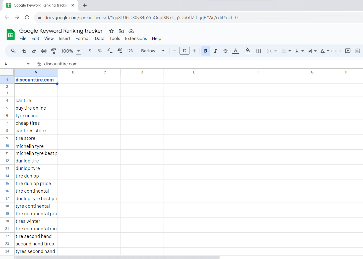
Step 1: Open a new Google Sheets and enter the website domain
Simply input the website domain you want to evaluate in the cell A1, in our case discountire.com.
Step 2: Input the keywords in the 1st column
For performance concerns, we recommend you to start with a maximum of 50 keywords. Simply add them in a column, as shown here:
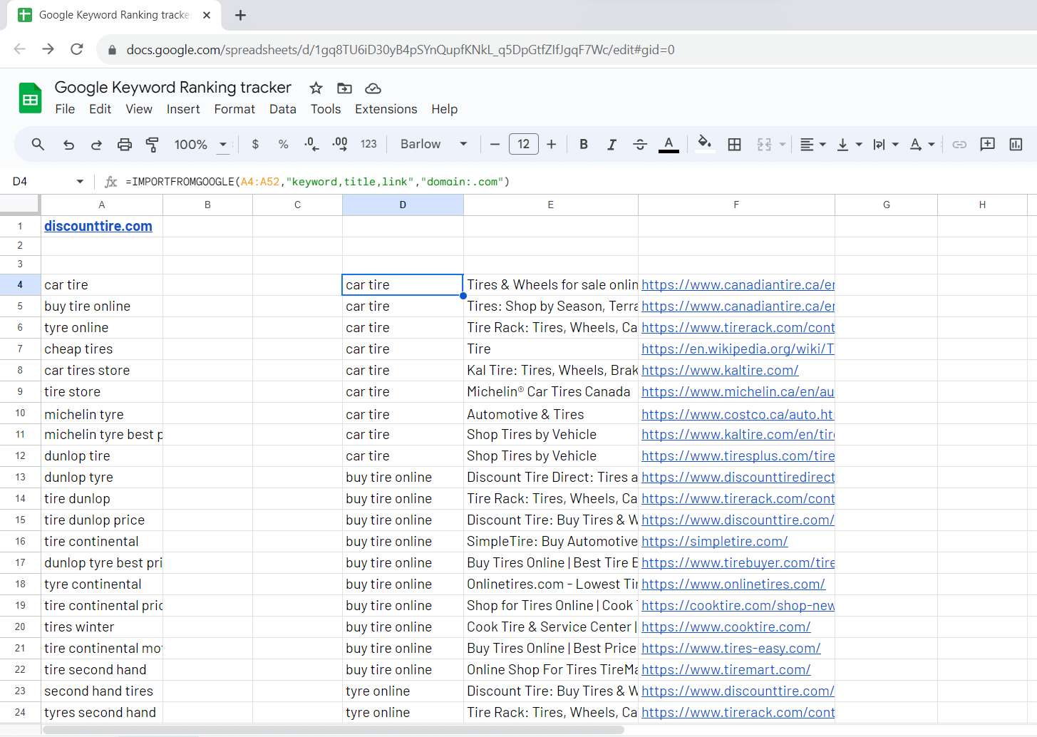
Step 3: Use the =IMPORTFROMGOOGLE() formula to extract the Google Search results
For each keyword, we’ll extract the title and the link of each result.
This is how the IMPORTFROMGOOGLE formula should look like (simply make a copy of it in the cell D4):
=IMPORTFROMGOOGLE(A4:A52,"keyword,title,link","domain:.com")
Besides the 3 selectors we have entered (“keyword”, “title”, “link”), the “domain” option we added as the 3d parameter of the formula specifies the Google domain we want to retrieve the results from. If you need to get the Google results from google.de, then you should write “domain:.de”
After a few seconds, the first 10 organic results for eack keyword or query will get loaded in a table:
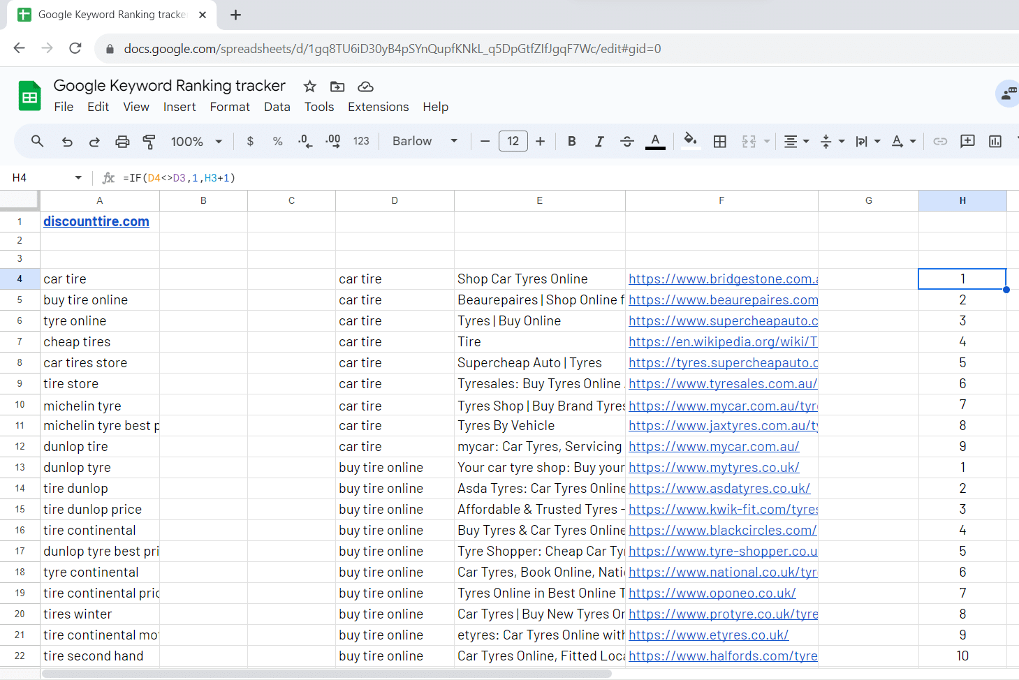
Step 4: Add the ranking of each returned result
The following formula entered in H4 and dragged down till the last row adds next to each result its Google ranking:
=IF(D4<>D3,1,H3+1)
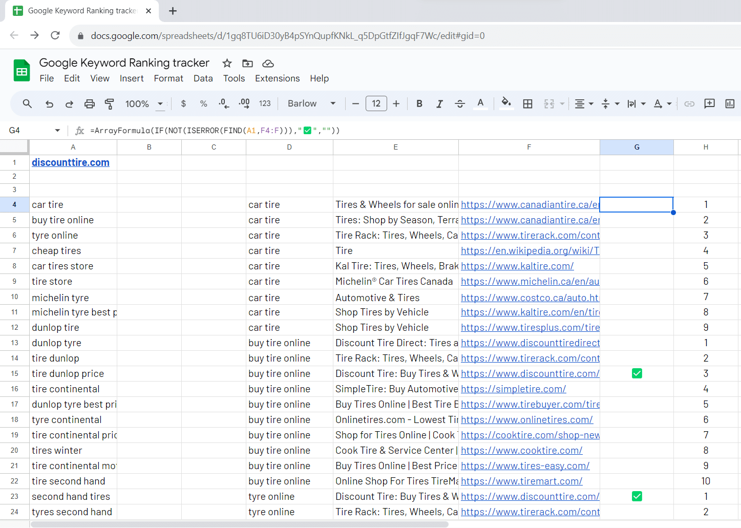
Step 5: Measure your website appearance
This formula adds next to each result a “✅” symbol indicating that your website (discounttire.com in our example) ranks for the keyword. The ArrayFormula ensures that the entire column F is processed at once.
=ArrayFormula(IF(NOT(ISERROR(FIND(A1,F4:F))),"✅",""))
Then, we’ll use another formula in B4 to filter values in column H based on matching keywords in column D and “✅” status in column G. It concatenates the filtered values, i.e. your website position(s) for each keyword – into a single text string separated by “; “. The IFERROR function ensures that if no matches are found or an error occurs, it returns an empty string.
=IFERROR(JOIN("; ",FILTER($H$3:$H,$D$3:$D=A4,$G$3:$G="✅")),"")
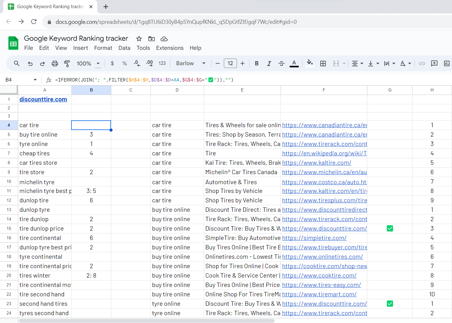
You have now a clear overview of the ranking of your website (in column B) for every single keyword.
Wanna more details? Let’s dive into the next step where we’ll create a summary table to disclose the number of keywords ranking in top 1, top 3 and top 10 results.
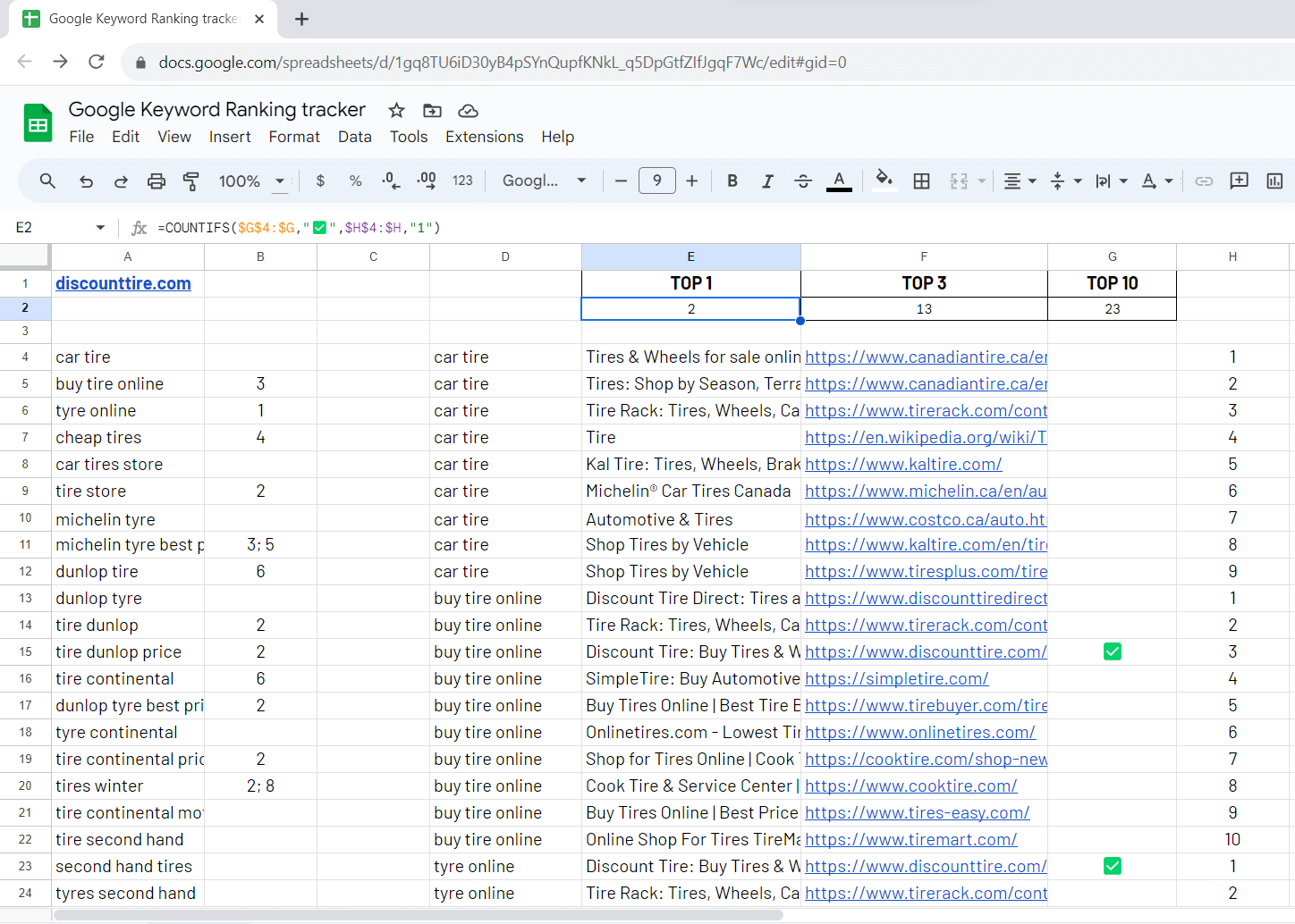
Bonus Step: build a simple ranking dashboard
This final formula uses the COUNTIFS function to count the number of rows where column G contains “✅” and column H contains the value “1”. It essentially counts the occurrences where both conditions are met simultaneously in the specified ranges.
=COUNTIFS($G$4:$G,"✅",$H$4:$H,"1")
Just adapt the formula as below to calculate the Top 3 and Top 10 website occurences:
TOP 3 formula:
=COUNTIFS($G$4:$G,"✅",$H$4:$H,"<=3")
Top 10 formula:
=COUNTIFS($G$4:$G,"✅",$H$4:$H,"<=10")
Needs to track the keywords over position 10?
Here’s your way to go: simply adapt the initial =IMPORTFROMGOOGLE() adding the num_results option! If you need to track the first 30 results for example, your formula should look like:
=IMPORTFROMGOOGLE(A4:A52,"keyword,title,link","num_results:30")
We’re done!
Now your Keywords Ranking Checker is ready, you can monitor your performances at your desired frequency. Whenever you open the spreadsheet and execute the =IMPORTFROMGOOGLE() formula, you get an updated view over your results!
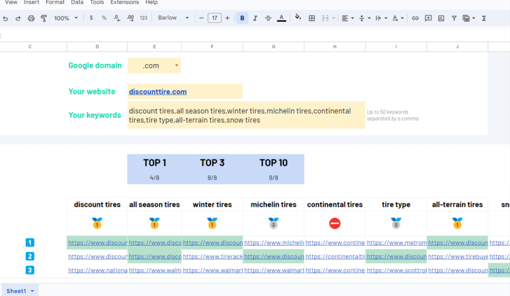
Our Free Google Sheets Template to track Keywords Ranking
If you just don’t want to follow the step by step above and build a Google Rank Checker from scratch, we got you covered!
Our Google Sheets Rank Checker template makes the job for you. All you have to do is to make a copy of it, then activate ImportFromWeb from the Extension menu and finally input your website and keywords.
We’d love to hear all of your feedback so that we can keep providing the best information on SEO monitoring combined with Google Search scraping! Feel free to reach out to us